The internal representation of spatial objects in R is quite complicated. You might already experienced this while searching for neat ways to plot maps of your data online. When everything you know consists of data.frames, lists, strings, and factors, you most probably had a hard time dealing with the answers presented there. But this is about to change. Once introduced to their representation, spatial objects and the corresponding plotting routines become as simple and straight forward as any other R objects.
Geospatial libraries and formats
There is a whole zoo of different libraries and formats dealing with spatial objects out there. So let’s make a quick guided tour and review the most important ones.
The GEOS packages, a C++ port of the JTS (Java Topology Suite), provides classes for basic geometric objects (like points, polygons, and lines) and definitions for operations performed on them (e.g. point in polygon or distance measures). In addition it is also able to import and export WKT (Well-known text) files, their binary presentation WKB, and GML (Graphical Markup Language) files. All these markup documents can represent both spatial objects and their coordinate reference systems.
Fortunately you don’t have to care about the various data formats for spatial data at all. Imagine the following scenario: Someone is providing you data in format A, which you have to transform into format B since your analysis is incompatible with the former one, and finally you have to hand your results to a collaborator in format C. In most fields, especially in data science itself, all those conversions are prone to cause a lot of trouble and force you to manually adjust the import and export procedures. But for spatial data you have the GDAL (Geospatial Data Abstraction Library). This very powerful and convenient package builds on top of GEOS and handles the reading and writing of 120 different raster and vector data formats used in geospatial applications. So whatever format you are dealing with, the GDAL package handles the import and provides you the data using the classes implemented in GEOS.
Our last main ingredient is the CRS (Coordinate reference system) describing the projection of a spatial object onto a map and its transformation into other CRS. This is quite important because a coordinate is basically nothing but a number. Without a reference placing them on a map those numbers are meaningless. Well, this might seems a little bit trivial since the usage of the equator, the prime meridian, and sea level are so common. But think about it. Due to the climate change the mean sea level is rising. So does the altitude of things decrease? As it turns out not even the prime meridian is at a latitude of exactly zero on GPS receivers. Therefore we need reference systems. Of course there are dozens. Some of them only span the entire world, some just specific countries, and others are tailored to the need of specific software and companies. We will stick to the most popular WGS84, which covers the whole globe.
As a matter of consistency, operations involving objects using different CRS are usually prohibited. Thus, we need the PROJ.4 C-library to handle both the transformation between the different systems and the actual projection of the spatial information onto a map.
Geospatial packages in R
The implementation in R looks quite similar. But here it is the sp package providing the classes and definition of the underlying spatial objects. Since most (if not all) R packages focusing on handling and plotting spatial objects are relying on this one, you can very easily interconnect various packages in your analysis making R an ideal language to work with this kind of data. So even if you are a R user but don’t plan to work with spatial objects, checking out this short introduction into the different classes and methods for spatial data is still a good idea.
Next we have the rgdal and the rgeos package. As you might already guess, they are both wrappers around the corresponding libraries. But remember, it’s still the sp packages providing the definitions of the spatial objects. So whenever you import some spatial data using the rgdal package it reads it with the standardized GEOS API and directly converts these objects into the classes implemented by the sp package.
For displaying our results we basically have three different options: the ggmap, tmap, and leaflet package. I will cover all them this blog post.
Worth mentioning are also the two package maps and maptools for providing different tools to manipulate spatial objects and the sf package. The latter is supposed to provide a more simple implementation of spatial objects and cover the functionality of the sp, rgdal, and rgeos package. But it is still under active development.
Installation
In order to install all those aforementioned R packages, you have to have some additional libraries installed on your system first.
# In Debian-based distributions.
sudo apt update
sudo apt install libjq-dev libv8-3.14-dev libprotobuf-dev libgdal-dev libproj-dev libudunits2-dev
Depending on which distribution is running on your computer, you might
have to download and install a more recent
GDAL version in order to install
the tmap package. If you were successful in installing it
using install.packages( "tmap" ), skip the following code
chunk.
# In case your system's repositories provide a GDAL package too
# old for the R packages above, you have to install a newer one
# from source.
# Download (into a folder you neither move, rename, or delete!)
wget http://download.osgeo.org/gdal/2.2.2/gdal-2.2.2.tar.gz
# Extract the folder
tar -xf gdal-2.2.2.tar.gz
cd gdal-2.2.2
# Run the ./configure script to tell the package all your local
# libraries, programs, and configurations
./configure
# Compile the source code
make
# Install the compiled code
sudo make install
Now we can load all the required packages into our R environment.
library( stringr )
library( dplyr )
library( tidyr )
library( rgdal )
library( maptools )
library( ggmap )
library( tmap )
library( OpenStreetMap ) # For more apealing visualization
library( leaflet )
Import and preparation of our data
Import
Firstly, we will download the polygons of the election districts.
## Download the files into a separated folder created in the current one.
download.folder <- "bundeswahlleiter/"
if ( !dir.exists( download.folder ) ){
  dir.create( download.folder )
}

## This URL contains all the geographical information.
election.districts.url <- "https://www.bundeswahlleiter.de/dam/jcr/f92e42fa-44f1-47e5-b775-924926b34268/btw17_geometrie_wahlkreise_geo_shp.zip"
## For convenience reason let's split the URL at all '/'. This way
## we can directly access the file name.
## Download
election.districts.url.split <- str_split(
    election.districts.url, "/" )[[ 1 ]]
download.file( url = election.districts.url,
              destfile = paste0( download.folder,
                                election.districts.url.split[ 7 ] ),
              method = "wget" )
## Extract the data for the election districts
unzip( paste0( download.folder, election.districts.url.split[ 7 ] ),
      exdir = download.folder )
The data format our polygons are provided in is the so called Shapefile. It is a vector format incorporating associated attribute information and features a number of actual files (the mandatory ones are marked with ’m’).
- .shp (m): Main shape file providing the coordinates for the different geometries
- .shx (m): Provides indices for the geometries
- .dbf (m): Holds the attribute information for the each spatial objects in separated columns
- .cpg: Specifies the code page/character set used for the encoding of the attributes
- .prj: Provides the CRS and the projection information in WKT
- .sbn/.sbx: Binary spatial indices of the features.
- .shp.xml: Contains geospatial metadata
You see, the term ‘Shapefile’ is quite counterintuitive since it consists of several files at ones.
Now we import the Shapefile into the R environment using the rgdal package.
## Import all the spatial information into one single data object.

## https://github.com/tidyverse/ggplot2/wiki/plotting-polygon-shapefiles
election.districts <- readOGR( dsn = paste0( download.folder, "." ),
                              layer = "Geometrie_Wahlkreise_19DBT_geo" )
Handling spatial objects in R
The election.districts object is not an ordinary R object like a
list or data.frame, as already noted, but of a special spatial class
provided by the sp package. It sure builds on top of those
fundamental classes, but it’s defined using the more strict S4 object
class. Thus, we aren’t able to use the name() function to access the
names of all its components and can’t access those using the $
symbol either. Instead of list elements, S4 based objects consist of
different slots accessible using @ symbol. You can get the
names of all available slots using the slotNames() function.
For our election.districts objects we care most about the polygons slot containing a list of all the different polygons consisting of the longitude and latitude coordinates of all their vertices and some metadata as well as the data slot holding a data.frame with the numbers and names of the individual election districts and the numbers and names of the corresponding states. The latter is also called an ‘attribute table’.
slotNames( election.districts )[1] “data” “polygons” “plotOrder” “bbox” “proj4string”
## Slot names of the first polygon stored in election.districts
slotNames( election.districts@polygons[[ 1 ]] )
[1] “Polygons” “plotOrder” “labpt” “ID” “area”
## ID of the first polygon
election.districts@polygons[[ 1 ]]@ID
[1] “0”
## First rows of the data slot
head( election.districts@data )
WKR_NR LAND_NR LAND_NAME WKR_NAME 1 01 Schleswig-Holstein Flensburg – Schleswig 2 01 Schleswig-Holstein Nordfriesland – Dithmarschen Nord 3 01 Schleswig-Holstein Steinburg – Dithmarschen Süd 4 01 Schleswig-Holstein Rendsburg-Eckernförde 5 01 Schleswig-Holstein Kiel 6 01 Schleswig-Holstein Plön – Neumünster
As you can see, the ID of each polygon/election district matches the name of the row (leftmost digit) of the data.frame stored in the data slot. In order relate it using the number of the election districts later on, we will have to increment (add 1) the IDs once. For a more thorough introduction to the S4 object class see the object-oriented chapter of Hadley’s advanced R book.
Importing the cleaned results of the election
Now we will import the results of the election we cleaned during the previous blog post into our current R environment. Note: we will use the last version of the data.separated object renamed to election.results. It’s a little bit inconsistent, but I decided to give it a more descriptive name to make things more clear within this and all following posts.
download.file( url = "https://github.com/theGreatWhiteShark/blog-resources/blob/master/coding/bundestag-election/election.results.RData?raw=true",
              destfile = paste0( download.folder,
                                "election.results.RData" ) )

## Load the cleaned results of the election
## Include a link to Github!
load( paste0( download.folder, "election.results.RData" ) )
Selecting the results we want to display
In this example we will work again with the preliminary total number of second votes for the leftists and another party called “Die Partei”.
## Exclude the states (since they cause the
## election.district.number to be not unique )
election.results.no.states <- filter( election.results,
                                       state.number != 99 )

## The amount of 2nd votes for the leftists (die Linke)
counts.leftists.second.vote <-
  filter( election.results.no.states,
         confirmation.status == "Vorläufig" &
         type.of.vote == "Zweitstimmen" &
         party == "DIE LINKE" )

## The amount of 2nd votes for die Partei
counts.partei.second.vote <-
  filter( election.results.no.states,
         confirmation.status == "Vorläufig" &
         type.of.vote == "Zweitstimmen" &
         party == "Partei für Arbeit, Rechtsstaat, Tierschutz, Elitenförderung und basisdemokratische Initiative" )
Plotting
Generally speaking it is possible to use the base plot() function
for plotting your polygons and to add additional layers representing
the information you want to display.
plot( election.districts )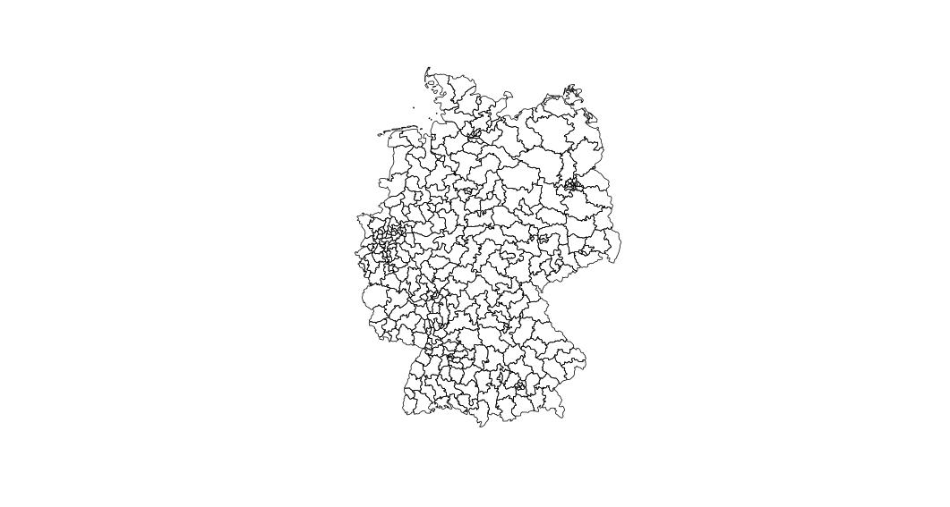
But I would highly recommend using more advanced packages instead.
In this tutorial I will cover the three main packages concerned with plotting maps: the ggmap, the tmap, and the leaflet package. So which one of these serves your needs best?
The ggmap package builds on top of ggplot2, which features a very intuitive way of handling your data and enables you to display loads of information using as few lines of codes as possible. Since ggplot2 should definitely be your package of choice for generating plots in R, it’s most convenient to add a layer of tiles to your existing plot using the ggmap package. But at the moment of writing the package is just badly implemented and a lot of things do not work. The broken OpenStreetMap support also seems to be a feature and not a bug. Nope. If all you want is to draw polygons, points, and lines, it’s a good idea to stick with the ggplot2 package. If you, instead, want to add tiles (parts of an actual map, like e.g. OpenStreetMap etc.), I would recommend the use of the tmap package.
tmap is based on the same Grammar of Graphics as ggplot2, is also structured using layers and aesthetics, and tries to provide the same syntax as the latter one. You’ll have many different themes of maps and ways to modify your results and the package itself is quite intuitive.
The leaflet package, on the other hand, takes things a few steps further. Using the htmlwidgets package it provides an interactive, JavaScript-based browser application. If you just want to produce some nice plots, this one is clearly over the top. You actually have less flexibility to manipulate the appearance of the map since you are relying on a R wrapper around the JavaScript package leaflet. But if you have high dimensional data to explore, this package can significantly ease the pain of extracting knowledge from your data set.
Plotting using ggmap
Since the ggplot2 package and its handling goes beyond the scope of this post, I would recommend you to either have a look at Hadley’s short but comprehensive introduction or to read over the code without a thorough understanding of what’s going on.
As a brief summary: The code for the ggplot2 package is structured in layers. We will print the tiles, the polygons etc. layer after layer on top of each other. All arguments for the functions producing e.g. lines or points can take two different types of input. Either one single constant number or string or a whole vector. The latter can hold numerical or character values and is called an aesthetic. Using those we can e.g. make the alpha value of each polygon to alter according to the number of votes or pick the color of the election district according to the party, which received the majority of votes.
The first thing we have to do when dealing with the ggmap or ggplot2 package is to convert our data into a data.frame. Spatial data formats are not supported.
## Converting the spatial object into a data.frame better suited
## for the 'ggplot2' package.
election.districts.df <- fortify( election.districts )
The resulting data.frame contains a separate row for each of the vertices containing the columns longitude, latitude, id, and group among others. The group column is used to associate all points to a distinct polygon and the id specifies the name of the corresponding row in the election.districts attribute table. To obtain the numbers of the election districts, which we need to relate the points to the election results, we have to increment the id column ones.
## Convert the IDs of the polygons to the same key used to
## identify the election districts.
election.districts.df$election.district.number <-
  as.numeric( election.districts.df$id ) + 1
Now we can relate the election results to the points constituting the election districts.
## Add the counts to all points of the corresponding polygons
election.districts.df <- left_join( election.districts.df,
                                   counts.leftists.second.vote,
                                   by ="election.district.number")
For the final plot we first get map tiles we will use as a basis for
our map with the get_map() function. But be careful: this one is
quite buggy! The true boundaries of the supplied polygons do not
work. So instead we have to adjust them carefully by hand.
Afterwards we’ll plot the districts on top of the tiles.
## Download map tiles. Be careful: this interface is quite buggy!
## The true boundaries of the supplied polygons do not work. Instead
## One has adjust the boundaries careful by hand.
map.tiles <- get_map( location = #bbox( election.districts ) )
                        c( left = 0, bottom = 47,
                          right = 20, top = 56 ) )
## Plotting the polygons on top of the map tiles.
ggmap( map.tiles ) + geom_polygon( data = election.districts.df,
                        aes( x = long, y = lat, group = group,
                            alpha = counts ),
                        color = 'black', fill = '#df0404' ) +
coord_quickmap() + theme_minimal() + xlab( "" ) + ylab( "" ) +
  scale_alpha_continuous( guide = FALSE )
## 'coord_quickmap()' ensures the axis to be of the right ratio
## to prevent a stretching of the displayed map.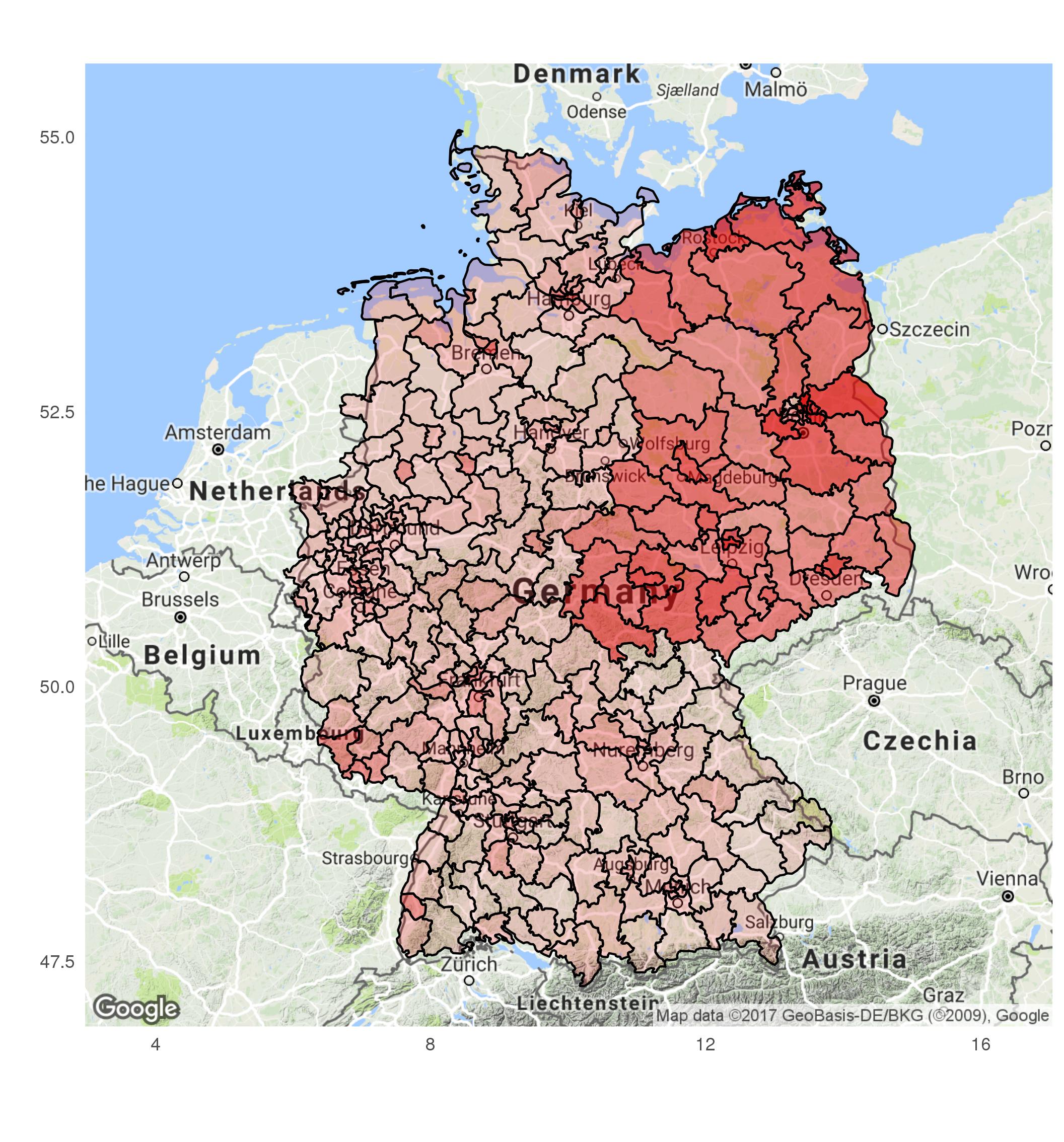
Plotting using tmap
In contrast to the ggplot2 package tmap sole purpose is to neatly visualize maps. Its most natural class to work with is not the data.frame, but spatial objects provided by the sp package. Therefore in this approach we will relate the extracted number of votes to the attribute information of the spatial object election.districts itself.
Firstly, we have to rename the election.district.number of the data.frame holding the results to match the WKR_NR column in the data slot of our shape object. In addition also we have to change the format of our data. Since every row in the attribute table is related to a specific polygon, we have to add the election results for different parties in separate columns (instead of one with an addition column specifying the name of the party).
## Renaming the column
counts.leftists.districts <- mutate( counts.leftists.second.vote,
                                    WKR_NR = election.district.number,
                                    counts.leftists = counts )
counts.partei.districts <- mutate( counts.partei.second.vote,
                                    WKR_NR = election.district.number,
                                    counts.partei = counts )
## Extracting only the relevant information
counts.leftists.districts <- select( counts.leftists.districts,
                                    WKR_NR, counts.leftists )
counts.partei.districts <- select( counts.partei.districts,
                                  WKR_NR, counts.partei )
## Combining the results by adding them into different columns.
counts.districts <- left_join( counts.leftists.districts,
                              counts.partei.districts,
                              by = "WKR_NR" )
counts.districts <- select( counts.districts, WKR_NR,
                           counts.leftists, counts.partei )
## Join the information about each polygon with the number of votes
## by the unique number of the election district.
election.districts@data <- left_join( election.districts@data,
                              counts.districts,
                              by = "WKR_NR" )
This may sounds quite frustrating and the resulting object is not ‘clean’ in the way we considered it throughout the last post. But different packages prefer different data structures and formats and in addition the libraries for ‘tidying’ data were established during the last years and some packages haven’t adapted (yet). But this is just how it is in open source languages.
Now let’s do a quick plot of the results. To do this with the least lines
of codes possible, the tmap package features the function qtm(),
which behaves similar as the qplot() function in ggplot2. But
this is not the only commonality. The tmap package as a whole is
very similar to ggplot2.
## Using the number of votes to fill the polygons with color
qtm( election.districts, fill = c( "counts.leftists", "counts.partei" ),
    fill.palette = list( "Reds", "Blues" ), cols = 2 )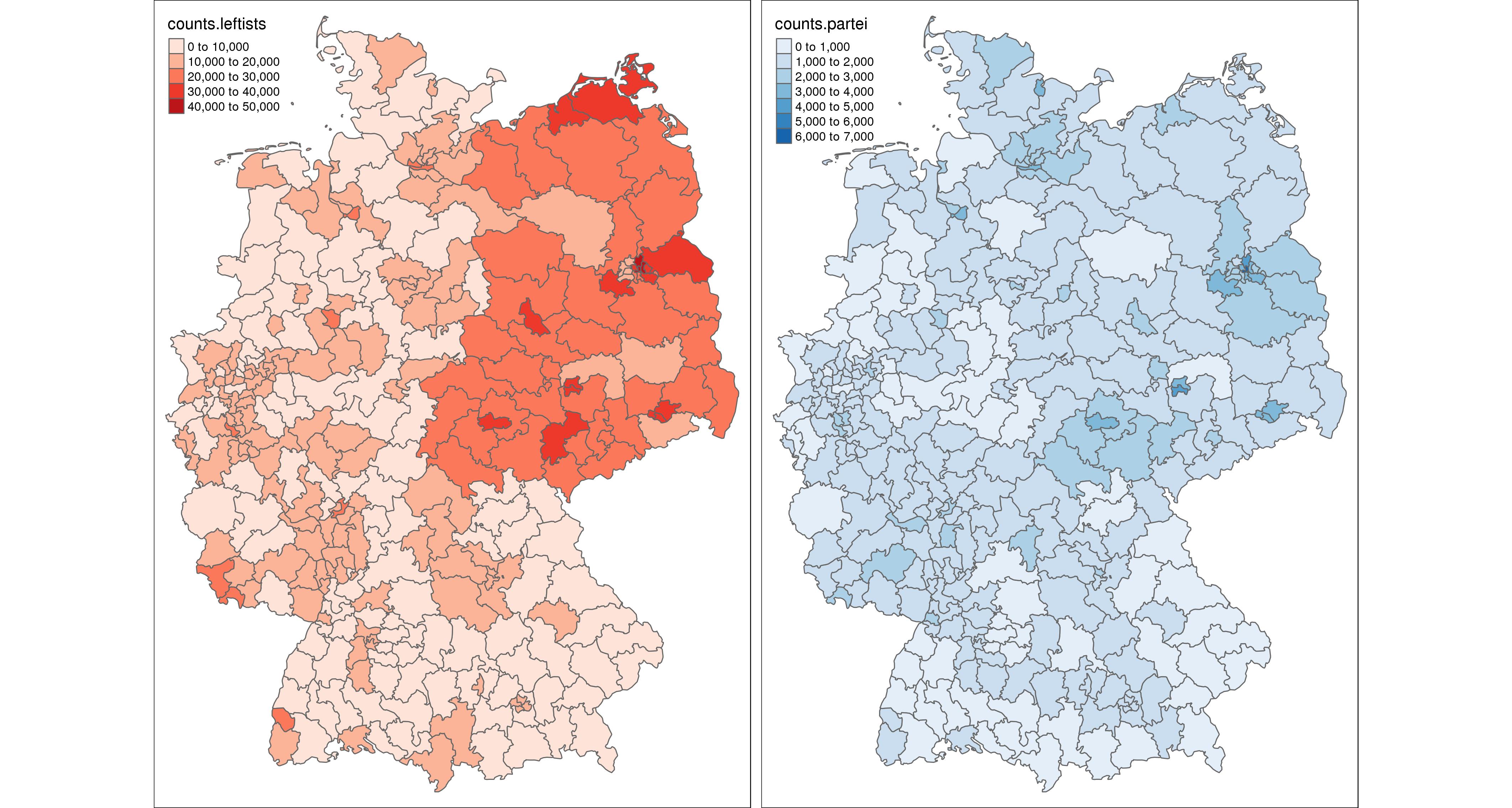
Next we will introduce map tiles provided by the OpenStreetMap project and plot the polygons of the election districts on top of them.
## Using the more verbose version of the writing code of the tmap package
tm_shape( tmaptools::read_osm( bbox( election.districts ) ) ) +
  tm_raster() + tm_shape( election.districts ) +
  tm_polygons( "counts.leftists", palette = "Reds", alpha = .5,
              fill.title = "Number of second votes for the leftists" )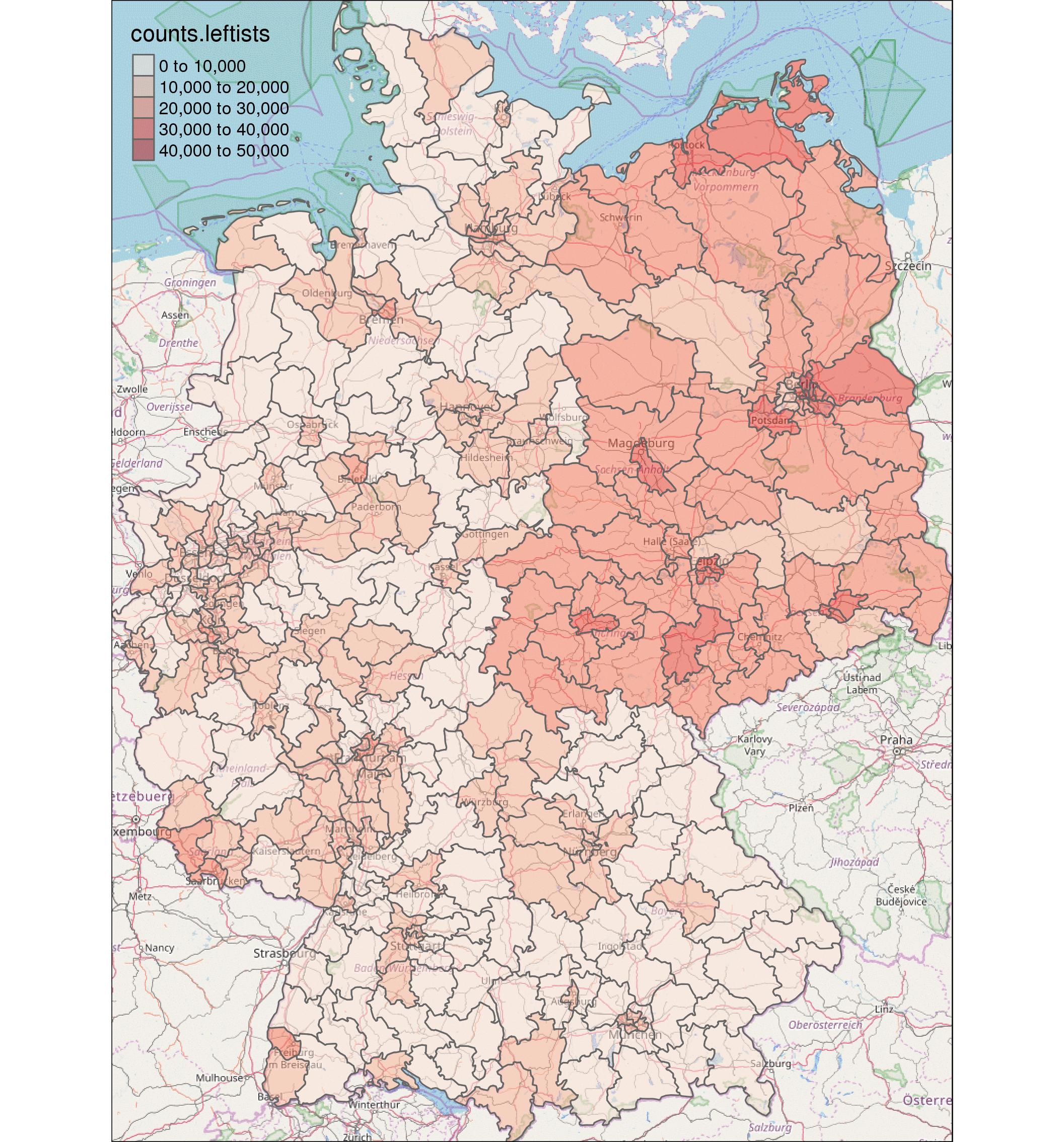
The tmap package features two different drawing modes. Beforehand we were using the plot mode generating highly customizable maps in X11 device windows. Alternatively, we can use tmap as a wrapper around the JavaScript package leaflet via the view mode.
## Displayed in the browser using leaflet package
tm_shape( tmaptools::read_osm( bbox( election.districts ) ) ) +
  tm_raster() + tm_shape( election.districts ) +
  tm_polygons( "counts.leftists", palette = "Reds", alpha = .5,
              fill.title = "Number of second votes for the leftists" ) +
  tmap_mode( "view" )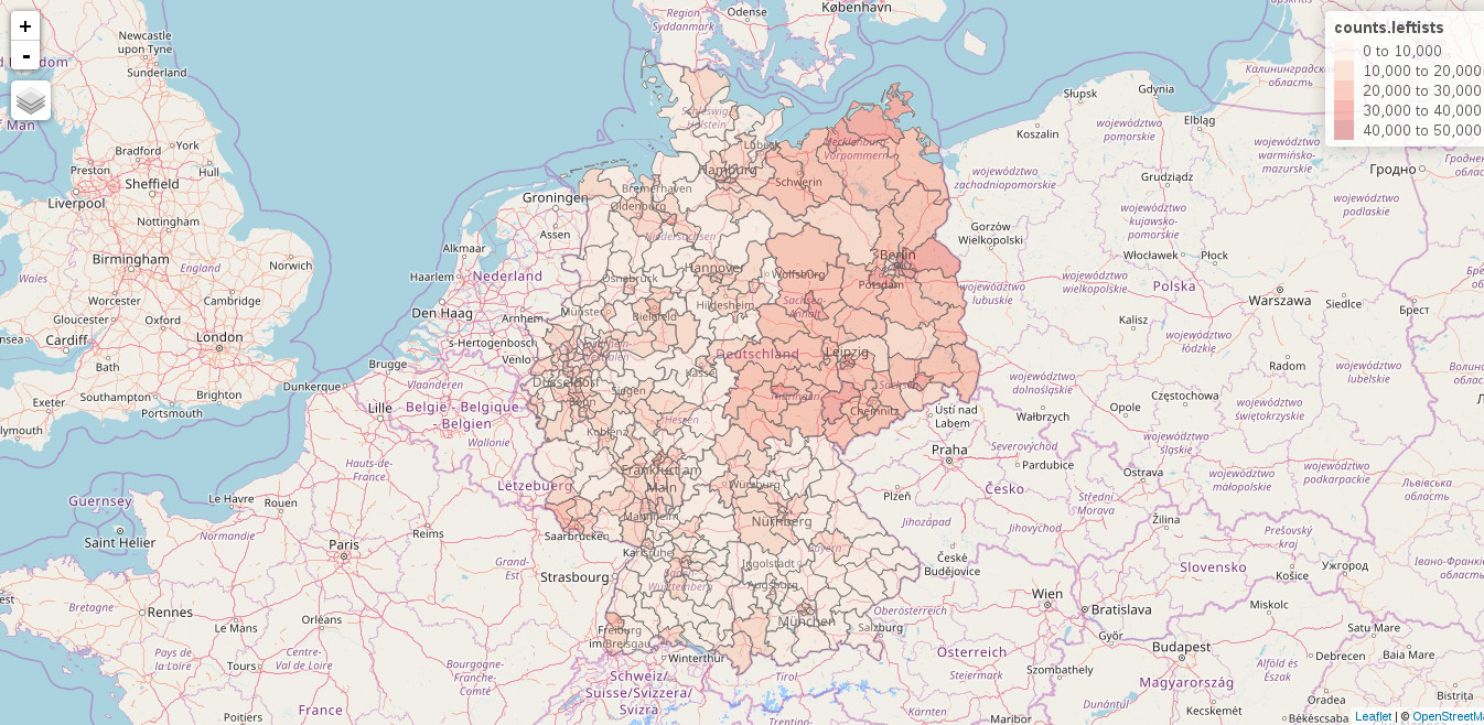
Now let’s plot something more advanced. For example the top 20 election districts ranked according to the number of votes for the leftists. To get a better feeling of the actual size of the individual districts we will use OpenStreetMap tiles for the background.
There are two main things to learn in this little example. Firstly,
functions for manipulating and cleaning data do not work on the
spatial object itself, but just on its attribute table. This might
seems kinda odd in the beginning since names( election.districts )
and head( election.districts$counts.partei act like they would
deal with the attribute table instead of the raw
polygons. In fact election.districts$counts.leftists is just a
shortcut for election.districts@data$counts.leftists. But such
shortcuts only exist for a small number of functions and in order to
assure compatibility of your code with future releases of packages,
it’s best practice to make all data assessments as explicit as
possible.
Secondly, there is the concept of factors in R. Factors are character vectors, which are only allowed to hold a predefined number of possible elements called levels. Okay. So why would someone need a second type of characters? Well, in the beginning of the R language, almost 25 years ago, this trick gave a huge burst in CPU and memory efficiency. As for today I would consider it to be a legacy component. But legacy or not, it’s still a commonplace. For a thorough introduction into factors see the corresponding section in Hadley’s R for Data Science book.
If we would just extract the rows of the spatial object holding the 20
largest values in the counts.leftists column and plot each of the
districts in their own subfigure separated by their unique name, the
order of the plots would be alphabetic. But this is not what we
intended. We want the order to be descending starting with the
district holding the largest number of votes. When we check out the
levels of the names of the election districts levels(
election.districts@data$WKR_NAME ) we see that they are indeed
ordered alphabetically. So we have to (you might already guessed it)
change the order of the levels to represent the top 20 election
districts.
## Displaying the election districts, which received the most votes.
## Extract the ordered names of the top 20 districts for the leftists.
top.20.districts <- as.character(
    arrange( election.districts@data,
            desc( counts.leftists ) )$WKR_NAME[ 1 : 20 ] )
## Selecting the spatial information for those 20 districts
election.districts.top.20 <- election.districts[
    election.districts@data$WKR_NAME %in% top.20.districts, ]

## Reordering the factor levels of the election districts according to
## the number of votes
election.districts.top.20@data$WKR_NAME <-
  factor( election.districts.top.20@data$WKR_NAME, levels = top.20.districts )

## Reordering of the factors according to the number of votes
tm_shape( tmaptools::read_osm( bbox( election.districts ),
                              type = "maptoolkit-topo") ) +
  tm_raster() + tm_shape( election.districts.top.20 ) +
  tm_polygons( "counts.leftists", legend.show = FALSE,
              alpha = .5, palette = "Reds" ) +
  tm_facets( "WKR_NAME", free.coords = TRUE ) + tmap_mode( "plot" )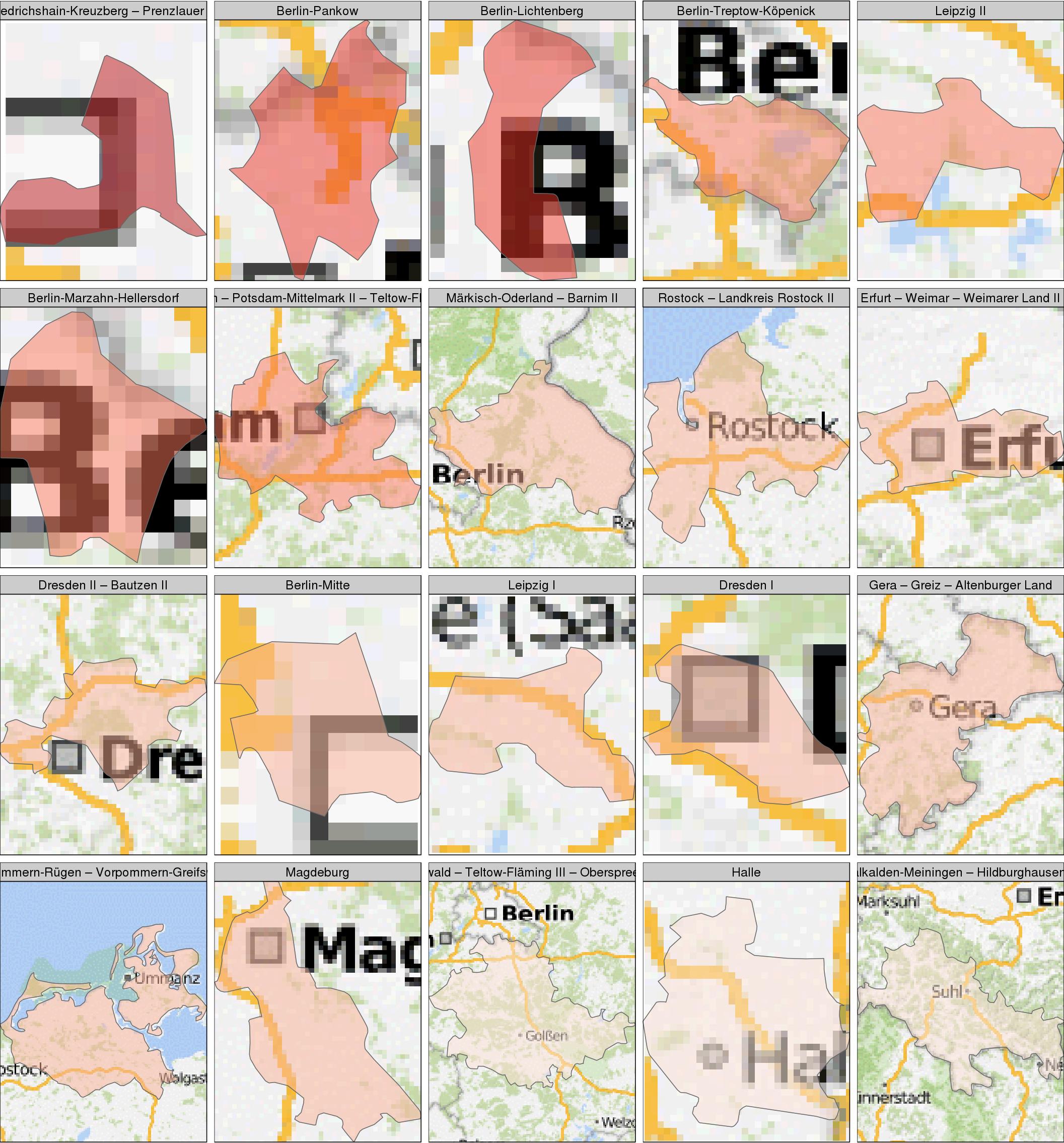
In our final example for the tmap package we will check out one of the many styles it is provides. We will plot both the number of votes for the leftist and die Partei in a classical map format you might remember from your textbooks in school. Since we do the plotting for two different columns/data sets, it’s best practice to avoid writing two very similar chunks of code, but to instead to write a function handling the job.
## Function for generating a classical plot.
classic.map <- function( column.name, color.palette, title ){
  ## In order to feature 'counts' as the heading of the legend, we have
  ## to generate/rename the corresponding column.
  election.districts@data$counts <- election.districts@data[,column.name]
  tm_shape( election.districts ) +
    tm_polygons( "counts", palette = color.palette ) +
    tm_compass( position = c( "right", "bottom" ),
               color.light = "grey90" ) +
    tm_style_classic( inner.margins = c( .04, .03, .02, .01 ),
                     legend.position = c( "left", "bottom" ),
                     legend.frame = TRUE, bg.color = "#f2d5b8",
                     legend.bg.color= "#f2d5b8", legend.bg.alpha = .3,
                     legend.text.size = .55, title = title,
                     legend.width = -.16,
                     earth.boundary = TRUE, space.color = "grey90",
                     sepia.intensity = .4, fontfamily = "Courier" )
}
## Generate the two plots (without actually plotting them)
map.leftists <- classic.map( "counts.leftists", "YlOrRd", "Leftists" )
map.partei <- classic.map( "counts.partei", "YlGnBu", "Die Partei" )
## Plot both figures next to eachother.
tmap_arrange( map.leftists, map.partei )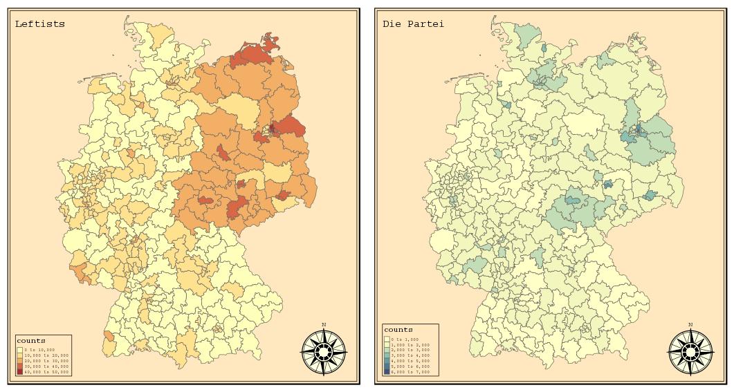
Plotting using leaflet
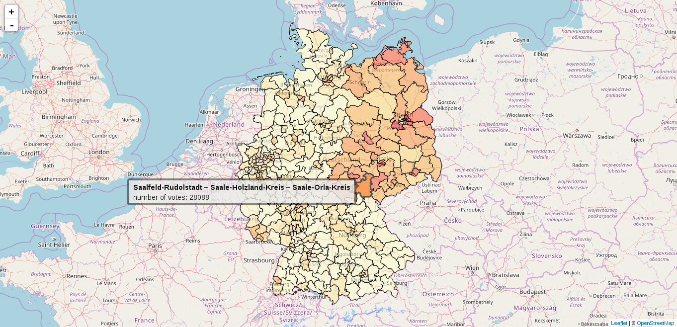
The leaflet package produces results quite similar to the ones generated in the view mode of tmap. But since the main purpose of leaflet is to be an easy to use wrapper around the JavaScript library leaflet it will be much more simple and convenient to tailor the resulting map to our needs.
All of the generated plots will be displayed in your default browser inside a new tab. So let’s make the most out of it and design our map to be as informative as possible. Therefore we will write a list of HTML codes called labels holding both the election districts names and the total number of votes. Whenever you hover your mouse over one of the polygons this label will be displayed. But of course not for the plot you can see below, which is just a screenshot (since I’m writing this as a static web page). So try it yourself!
## Defining a custom palette for the map.
color.palette <- colorBin( "YlOrRd",
                          domain = election.districts@data$counts.leftists )
labels <- lapply( sprintf(
    "<strong>%s</strong><br/>number of votes: %g",
    election.districts$WKR_NAME, election.districts$counts.leftists ),
    htmltools::HTML )

leaflet( election.districts ) %>%
  addProviderTiles( "OpenStreetMap" ) %>%
  addPolygons( data = election.districts,
              fillColor = ~color.palette( counts.leftists ),
              opacity = 1, color = "black", fillOpacity = .5,
              weight = 1,
              highlight = highlightOptions(
                  weight = 3, color = "#555", fillOpacity = .8,
                  bringToFront = TRUE ),
              label = labels,
              labelOption = labelOptions(
                  style = list( "font-weight" = "normal",
                               padding = "3px 8px" ),
                  textsize = "15px",
                  direction = "auto" ) )
To get the most out of the leaflet package I strongly recommend to use it in corporation with shiny. There you can have e.g. a widget with which you can select the parties, which results you want to display on the map. It’s a very powerful package and out of the scope of the post. Check out the app of my climex packages as a comprehensive example. So yes, you can host such little applications too using shiny-server.
Further reading
In case you are looking for further information about spatial objects in R and their visualization, be sure to check out tmap’s guide tmap in a nutshell, Robin Lovelace’ tutorial for creating maps in R, or this extended tutorial based on a book chapter of Robin Lovelace’s, Jakub Nowosad’s, and Jannes Muenchow’s Geocomputation with R (which is still work in progress).