Thanks to loads of publicly available data it’s possible to get further insight into the past and current state of the world, as well as possible future perspectives. May it be for professional reasons as a data scientist or just out of pure curiosity, using modern statistical computer languages all of us are capable of obtaining those insights.
Introduction
It’s often said that as a data scientist you spend 80% of your time not on your analysis but on the data itself: 40% on finding the right data and 40% on cleaning it. While for small examples (like this one) it’s certainly true, for large analysis including many hypotheses, machine learning, and/or model-based approaches in my experience the analysis gets more dominant. But nevertheless, your data will always plays a central role and thus for data science I would highly recommend choose a programming language focusing on handling data over a general purpose one.
Which computer language should I use?
If you duckduckgo Data science programming language or lend an ear to people working with data you quickly realize it boils down to four different languages, which are free and open source: R, Julia, Scala, and Python. While the first two are statistical languages designed around the handling of actual data, the latter are general purpose languages featuring nice packages for doing the same job. Using the statistical ones you can start more fast and the overall handling of object within the language is more convenient. The general purpose ones, on the other hand, enable you to solve problems beyond those of a data scientist.
My recommendation is: choose whatever you like! All of those four languages are awesome, come with tons of documentation and tutorials, and already produced endless helps and advises on pages like Stackoverflow. High-level computer languages featuring interpreters are all quite alike and since we are not digging the very roots of the language you will be able to perform this analysis in all four of them in no time. In addition your ability to collaborate with other people or to integrate their code into yours will increase tremendously as soon as you are able to read and write simple lines of code in as many languages as possible.
In this post I will choose R. I use it over Julia since the latter was brand new and didn’t had that much momentum when I started working with data as port of my PhD. But it’s supposed to be more fast and robust than R and I’m already looking forward to do some projects using it in the near future. Scala is more of a web-centered language and Python does not feature specialized time series analysis packages I need in my regular line of work. But let me stress it again: they are all perfectly suitable for this example.
Sometimes people try to argue for the language they are most comfortable in to be the best in the world. Be better than those people. Be a multi-lingual!
The problem at hand
In this little example we will download the results for all election districts in Germany and convert them into a format we are comfortable working with. Since the data will be high-dimensional (the number of votes for each individual party in all election districts) we will display the information using maps. Therefore we also need to download and handle the shape files of all the election districts.
For a more thorough introduction into data science using R have a look at Hadley’s corresponding book.
Download the data
First of all we have to load a number of R packages. If you don’t
have them installed yet, use the install.packages() function to do
so.
In addition you need two non-standard Linux packages in order to install the R packages handling your map data.
# On Debian-based and Ubuntu distributions
sudo apt update
sudo apt install libgdal-dev libproj-dev
All remaining code has to executed in a R shell.
## Loading the required packages
library( dplyr )
library( tidyr )
library( tibble )
library( readr )
library( stringr )
library( rgdal )
library( rgeos )
library( maptools )
library( ggplot2 )
Next we will download the results of the election provided by bundeswahlleiter.de into a separate folder.
## Save all data in a separate folder (within the current one)
download.folder <- "bundeswahlleiter/"
if ( !dir.exists( download.folder ) ){
  dir.create( download.folder )
}
## URL pointing to the file containing the results for all of Germany.
data.election.url <-
  "https: //www.bundeswahlleiter. de/dam/jcr/72f186bb-aa56-47d3-b24c-6a46f5de22d0/btw17_kerg.csv"

data.election.path <- paste0( download.folder, "btw17_kerg.csv" )
## Download
download.file( url = data.election.url,
              destfile = data.election.path,
              method = "wget" )
Tidy the data
To handle and clean the data we will use packages from the so-called tidyverse, a new school approach of doing things in R. Most of those packages are quite handy (expect of the annoying pipes provided via the magrittr package).
The keys of the individual columns of the data are provided in a hierarchical structure. The first header iterates through the individual parties, the second through the type of vote, and the last through the confirmation state. Therefore the header can not be simply read from file but has to be added by hand. But before jumping right into the import functions of your programming language better take one or two minutes and just have a look at your data using a simple editor. What’s the structure of the header? Which information is contained? What’s the shape and data type of the columns? … Getting a feeling for your data is quite important.
The overall goal is to produce a clean data set. Though, there is no universal definition of what is clean or not and each field has it’s own particular view on this topic, we will use the format preferred by the tidyverse (and by myself). In there we have a separate row for each observation and a separate column for each additional information or attribute. So we want to have a single column containing the number of votes and additional columns specifying the name of the election district, type of vote, party etc. corresponding to this individual value. Using this format and descriptive column names it will be incredibly straight forward to filter the election results afterwards.
Disclaimer: The data is quite fresh and hot. So if either the download URL or the structure of the data changes, please leave a comment. I’ll try to adjust the code as soon as possible. :)
Import data
Next we will import the election results into R.
data.pure <- read_delim( data.election.path, delim = ";",
                            col_types = cols( .default = col_integer(),
                                             X2 = col_character() ),
                            col_names = FALSE, skip = 5 )
There are a bunch of warning messages for the command above. But as far as I can tell all the data is present and this is what really matters. We aren’t writing a package here, so let’s be quick (and maybe a little bit dirty). .
There are some rows in the original data featuring only one single semicolon. Thus they result in rows consisting of only NA entries. NA is R’s acronym for “not available” and represents missing data. These have to be removed. Since each election districts must have a unique name, we will use the second column to search for and remove those NA rows.
data.pure.na.row <- which( is.na( data.pure[[ 2 ]] ) )
data.pure <- data.pure[ -data.pure.na.row, ]
The presence of such artifacts only becomes apparent when you continuously inspect your data. The more you trust the people providing your data and the algorithm you use for importing, the more busy you will be finding and fixing bugs in your analysis.
Extract header
Now we have to extract all the strings composing the header and combine the hierarchical structure into a single key per column in order to correlate them later on.
data.header <- readLines( data.election.path, n = 5 )

## Combining the hierarchical header structure into a single key per
## column.
data.header.1 <- str_split( data.header[ 3 ], pattern = ";" )[[ 1 ]]
data.header.2 <- str_split( data.header[ 4 ], pattern = ";" )[[ 1 ]]
data.header.3 <- str_split( data.header[ 5 ], pattern = ";" )[[ 1 ]]
The headers of the higher levels (1 and 2) of the hierarchy leave the key to a column empty whenever it holds the same string as the previous one. Therefore we have to write a function filling those gaps.
fill.header <- function( string.vector ){
  for ( ll in 2 : length( string.vector ) ){
    if ( string.vector[ ll ] == "" ){
      ## Check whether the previous entry contains a string. We will
      ## only fill the vector in downward direction.
      if ( string.vector[ ll - 1 ] != "" ){
        string.vector[ ll ] <- string.vector[ ll - 1 ]
      }
    }
  }
  ## The last column is an artifact
  string.vector[ length( string.vector ) ] <- "NA"
  return( string.vector )
}
data.header.1.filled <- fill.header( data.header.1 )
data.header.2.filled <- fill.header( data.header.2 )
data.header.3.filled <- fill.header( data.header.3 )
data.header.combined <- str_c( data.header.1.filled,
                              data.header.2.filled,
                              data.header.3.filled, sep = '_' )
The first three elements of our adjusted header won’t be needed or touched when reshaping the data. Therefore we will give them a proper name and overwrite the column names of the imported data afterwards.
data.header.combined[ 1 ] <- "election.district.number"
data.header.combined[ 2 ] <- "election.district.name"
data.header.combined[ 3 ] <- "state.number"

## Now we can assign the column names to our data.
colnames( data.pure ) <- data.header.combined
Reshaping the data
As an intermediate step, we write all the integer data representing the number of votes in one column called “counts” and all the names of the corresponding columns in another one called “party_type.of.vote_confirmation.status”. In the realm of the tidyverse this operation is called gathering and illustrated in greater detail in here.
data.gathered <- gather( data.pure,
                        4 : length( data.header.combined ),
                        key = "party_type.of.vote_confirmation.status",
                        value = "counts" )
Now we separate the attributes we combined in the header into
individual columns using the underscores. A number of vote V associated
with a key X_Y_Z in the “party_type.of.vote_confirmation.status”
column will now be associated with X in the “party”, Y in the
“type.of.vote”, and Z in the “confirmation.status” column. Again,
there is a tidyverse-specific name called separating and a further
illustration can be found in
here.
data.separated <- separate( data.gathered,
                           `party_type.of.vote_confirmation.status`,
                           into = c( "party", "type.of.vote",
                                    "confirmation.status" ),
                           sep = "_" )
Working with tidy data
Congratulations. Your data is clean! So what did we gained and was it really worth the effort?
Now you can search your data in a very intuitive way. Since every single bit of information is condensed in its own column, you just have to specify the ones you are interested in and use the others to search/reduce the data. So you specify the columns you are interested in and throw out the rows you don’t care about.
Imagine you want to know the preliminary number of second votes (direct votes for a specific party) for all parties in the election district called Hamburg. You just have to select the counts column and use all the other columns to search your data like a database.
## Tidyverse way of doing it
## Boiling your data down to the rows you are interested in.
votes.hamburg.filtered <- filter( data.separated,
                                 election.district.name == "Hamburg",
                                 confirmation.status == "Vorläufig",
                                 type.of.vote == "Zweitstimmen" )
## Extract just the name of the party and the number of votes.
select( votes.hamburg.filtered, party, counts )

## The oldschool way of doing it
votes.hamburg.filtered <- data.separated[
    data.separated$election.district.name == "Hamburg" &
    data.separated$confirmation.status == "Vorläufig" &
    data.separated$type.of.vote == "Zweitstimmen", ]
votes.hamburg.filtered[ , c( "party", "counts" ) ]
Or you are interested in all the election districts the party SPD obtained more than 200000 preliminary first votes in.
votes.for.the.spd <- filter( data.separated,
                            confirmation.status == "Vorläufig",
                            type.of.vote == "Erststimmen",
                            party == "Sozialdemokratische Partei Deutschlands",
                            counts > 200000 )
votes.for.the.spd$election.district.name
In addition you should always check for the validity of the results by comparing e.g. all data of one election district against the row in the corresponding .csv file we imported our data from.
filter( data.separated, election.district.name ==
                      data.separated$election.district.name[ 1 ]
      )$counts
But be careful about the encoding here! At least for me entering the names of the districts by hand didn’t worked for all of the them.
data.separated$election.district.name[1] == "Flensburg - Schleswig"[1] FALSE
This is caused by a different ‘minus sign’ in the data.
data.separated$election.district.name[1] == "Flensburg – Schleswig"[1] TRUE They appear to be identically but they are not!
charToRaw(data.separated$election.district.name[1])[1] 46 6c 65 6e 73 62 75 72 67 20 e2 80 93 20 53 63 68 6c 65 73 77 69 67
charToRaw( "Flensburg - Schleswig" )[1] 46 6c 65 6e 73 62 75 72 67 20 2d 20 53 63 68 6c 65 73 77 69 67
This is probably the case since I’m using a Linux machine and the document seems to be written in a Windows-based environment.
guess_encoding( charToRaw( str_c( data.separated$election.district.name,
                                 collapse = "" ) ) )
encoding confidence
1 UTF-8 1.0 2 windows-1252 0.3
Anyway. Most importantly the values do match and the tidying is complete.
Display the data
Of course we can just print our results as a table or vector but our data at hand is best displayed and interpreted using maps.
The handling of spatial data is an advanced topic and worth a post itself. That’s why I will just summarize the mere basics of generating a nice map using the ggplot2 package here and cover the topic of geographical data and their representation in the next post.
Download and import the shape data
First of all we need to download and extract the shape files of the election districts.
## This URL contains all the geographical information.
election.districts.url <- "https: //www.bundeswahlleiter .de/dam/jcr/f92e42fa-44f1-47e5-b775-924926b34268/btw17_geometrie_wahlkreise_geo_shp.zip"
## For convenience reason let's split the URL at all '/'. This way
## we can directly access the file name.
## Download
election.districts.url.split <- str_split(
    election.districts.url, "/" )
download.file( url = election.districts.url,
              destfile = paste0( download.folder,
                                election.districts.url.split[ 7 ] ),
              method = "wget" )
## Extract the data for the election districts
unzip( paste0( download.folder, election.districts.url.split[ 7 ] ),
      exdir = download.folder )
Now we import all the spatial information into one single data object. The shapes are stored as polynomials. We will extract all coordinate of their vertices and display them using a regular plotting engine. .
election.districts <- readOGR( dsn = paste0( download.folder, "." ),
                              layer = "Geometrie_Wahlkreise_19DBT_geo" )
## Converting the spatial object into a data.frame better suited
## for the 'ggplot2' package.
election.districts.df <- fortify( election.districts )
Relate the election results and the district geometries
Now we have two clean data sets. But those on their own are not really that helpful for generating the plots we are looking for. What we have to do now is to combine them. The technical term for those data sets is relational data.
In order to accomplish this task we need at least one key (column) to be present in both data sets. Since we did just imported the geometry of the individual election districts, it’s only natural to use their numbers. The object election.districts.df features a key called id which does the job but starts at zero. So we have to increment all its entries and rename the key.
## Convert the IDs of the polygons to the same key used to
## identify the election districts.
election.districts.df$election.district.number <-
  as.numeric( election.districts.df$id ) + 1
What we will do next is to take each district number of every coordinate combination (row) in election.districts.df and add all data from data.separated which rows feature the same value. But this is just one of many ways to relate your data sets.
As you might have already noticed when inspecting your data earlier: we have a problem. The election district numbers are not unique.
Unfortunately, the implicit assumptions you make about your data aren’t true more often than you think. Most of the time such issues are fixed after a short dive into your data. But keep in mind to frequently check your intermediate results or you may miss such glitches, which might even spoil your whole analysis.
In our case the states of Germany (a superset of the election districts) are listed as well. Not with distinct numbers in the election.district.number column, but with the one held by the district which appears first in the data. Since we have the key state.number and all states have their value set to 99, we can filter them out in no time.
current.election.no.states <- filter( data.separated,
                                       state.number != 99 )
In general we can combine the whole data sets. But in our small example we will focus on a specific information we want to display. Let’s say the number of preliminary second votes for the leftists (die Linke).
counts.leftists.second.vote <-
  filter( current.election.no.states,
         confirmation.status == "Vorläufig",
         type.of.vote == "Zweitstimmen",
         party == "DIE LINKE" )
## Select just the 'election.district.number' key and the
## 'counts' value (number of votes)
counts.leftists.second.vote <- select(
    counts.leftists.second.vote, election.district.number,
    counts )
This filtered set of rows and columns we now relate to the spatial information.
## Add the counts to all points of the corresponding polygons
election.districts.df <- left_join( election.districts.df,
                                   counts.leftists.second.vote,
                                   by ="election.district.number")
Finally, we will plot the results using ggplot2. This package and its underlying Grammar of Graphics ensures your plots to always look nice and should be your plotting package of choice in R. Since its handling and its layered structure is not that straight forward, let me just summarize the main things that happen in the next couple of line and point to Hadley’s chapter on Data Visualization.
We will separate the vertices of the individual polygons by the group aesthetic and plot all the districts separately within the same figure. Each one of them will be filled red and its alpha value (opacity) will represent the number of votes for the leftists.
ggplot() + geom_polygon( data = election.districts.df,
                        aes( x = long, y = lat, group = group,
                            alpha = counts ),
                        color = 'black', fill = '#df0404' ) +
coord_quickmap() + theme_minimal() + xlab( "" ) + ylab( "" )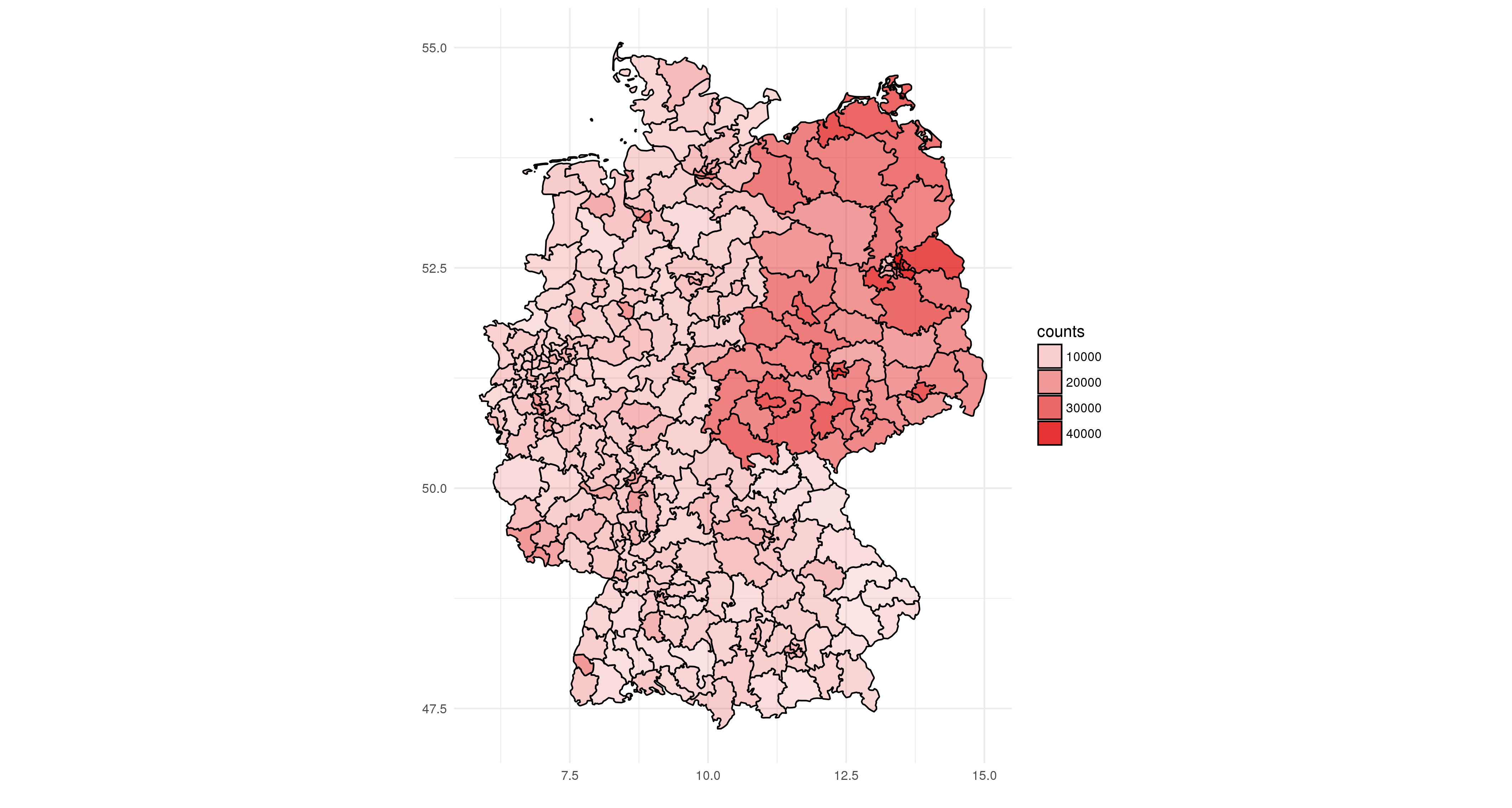
Cleanup
When all is said and done, you can delete the folder holding the downloaded data using the following command.
unlink( download.folder, recursive = TRUE )Preview
We have learned how to download, clean, and use the results of the 2017 election for the Bundestag. But what about the weird format of the shape files? And is it possible to plot the map in an even nicer fashion? Maybe in combination with an actual map using OpenStreetMap tiles or an interactive one showing the names of the states etc. when hoovering over it by mouse?
All this I will cover in the next post of this series. So stay tuned.