The Climex app is my longest and most comprehensive endeavor in the realm of programming and software development up to now. It started as a couple of wrapper functions in the beginning of my PhD in 2015 and is still (at the time of writing) under active development.
In this post I won’t explain the motivation and basics of the extreme value analysis (EVA), which can be found in the vignettes of the package, but its basic handling and the improvements it introduces.
Motivation
There are already a bunch of R packages for the fitting of extreme value distributions. So, why did I decided to write my own one?
Right from the start I wanted to perform EVA on a massive parallel scale by fitting the generalized extreme value (GEV) and generalized Pareto (GP) distribution to all stations within a country or region or to all grid points of a climate model/reanalysis data. But when apply the EVA to several hundreds of time series in parallel, I always encountered errors or numerical artifacts for at least a couple of them. Exchanging the fitting functions and packages helped for specific stations. But then again all packages produced errors; just for different stations. So I decided to dive into this topic and to write a package, which is more robust, fits my needs and permits a massive parallel application.
Improved fitting routines
The parameter estimation for the stationary GEV and GP distribution using the maximum likelihood method in an unconstrained optimization (done by all other R packages involving extreme value statistics) tends to produce numerical artifacts. This is due to the presence of logarithms in the negative log-likelihood functions and a limited range of shape values the maximum likelihood estimators are defined in. While yielding absurdly large parameter values or causing the optimization to fail when using the BFGS algorithm (in the extRemes package), the differences using the Nelder-Mead algorithm (all other packages, e.g. ismev) might be small, barely noticeable, and totally plausible. But they are still present and spoil your calculation.
In order to avoid those numerical artifacts, the augmented Lagrangian method is used to incorporate both the logarithms and the limited range of shape values as non-linear constraints. With this approach the optimization can be started at arbitrary initial parameter combinations and will almost always converge to the global optimum. Only for initial parameter combinations chosen very badly the algorithm can still produce artifacts. But an improved version of the already quite decent heuristics for choosing them will prevent it.
This solves two remaining problems of the extreme value analysis:
- The user does not have to worry about the numerical optimization anymore. It will produce the correct results in nearly all cases.
- The optimization itself becomes more robust and can now be used in
an massive parallel setting.
Error estimates of the return level
An important part of the extreme value analysis is to access the fitting errors introduced into the calculated return levels. The default way of obtaining them is to use the so-called delta method assuming normality of the log-likelihood function at the fitting result. This assumption, however, is not fulfilled in a lot of cases and is stronger violated the higher the shape parameter of the underlying GEV or GP distribution.
To nevertheless calculate a decent estimate of the fitting errors, the climex package introduces two statistical approaches, one based on bootstrap and the other one based on a Monte Carlo approach. In comparison to the calculation of the confidence intervals implemented in the extRemes package, the climex package calculates the standard deviation of the return levels. Since there are a lot of different sources of errors in the extreme value analysis, like too small block sizes, too low thresholds, or non-stationaries and/or correlations in the data, providing a confidence interval (CI) might the misleading for some users. All these additional errors are by no means included in the CI and have to be obtained in further studies to construct some appropriate CI of the calculated return levels.
Better error handling
Due to the use of either the Nelder-Mead or BFGS optimization algorithm, some time series will throw errors when fitted using the other R packages tailored for the extreme value analysis. When fitting 100 stations at once you can expect at least one of them to break your code.
In order to allow a massive parallel application of the extreme value analysis, the climex package features a more robust error handling. In addition, the improved fitting routine mentioned above is able to handle initial parameter combinations far more distant from the global optimum than feasible under any unconstrained routine.
Focused on handling time series
The fundamental object class handled in the climex package is the time series class xts or lists of class xts objects. This allows the user to harness all the additional functions tailored for the analysis of time series, e.g. those of the lubridate package. It also includes a couple of convenience functions often used within the extreme value analysis, like blocking, application of a threshold, declustering, deseasonalization etc.
To build a decent foundation of climatological data your analysis can rely on, I wrote the package dwd2r, which downloads large amounts of data from the FTP server of the German weather service (DWD) and converts them into a format usable within R. For more details see the corresponding post.
Shiny-based web application
Since it’s quite cumbersome to handle dozens, not to mention many hundreds of time series, I also wrote a Shiny-based web application in the package climexUI to perform the EVA on the individual series.
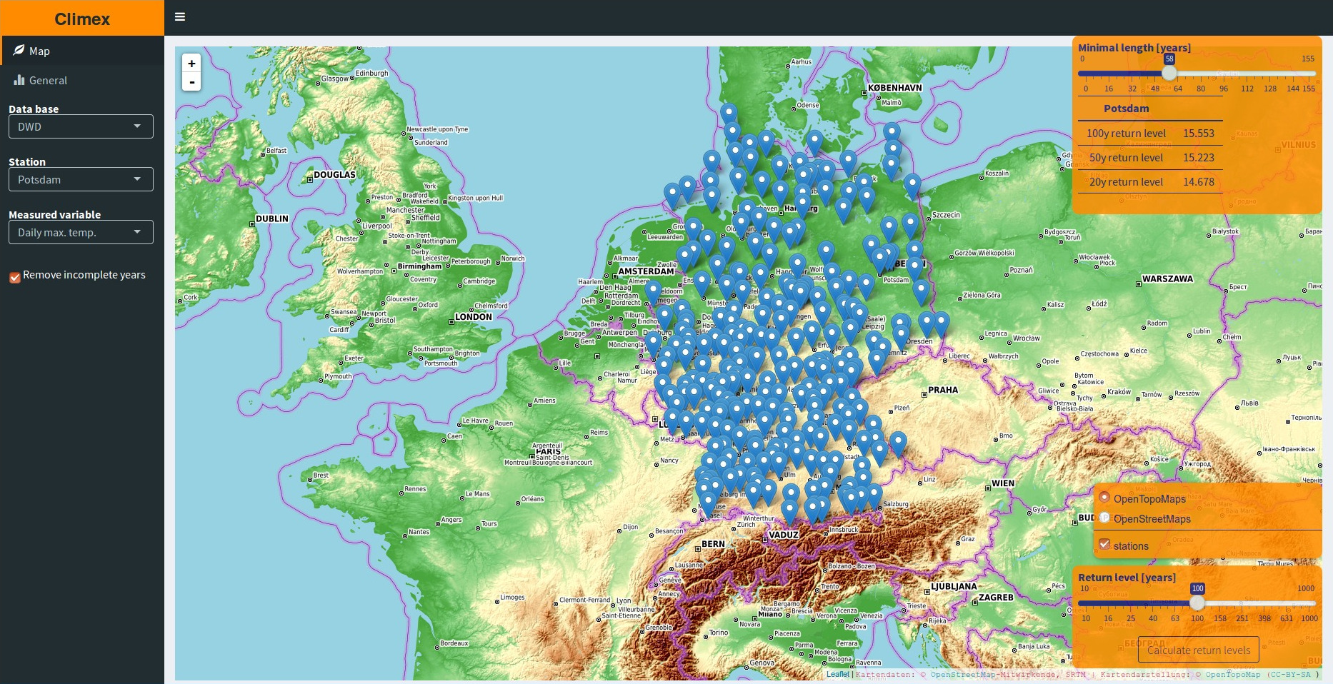
It features two different tabs. The first one holds a leaflet map the user can interactively choose the station she want to perform the analysis on from. Also the most important information concerning the chosen series is displayed in a box.
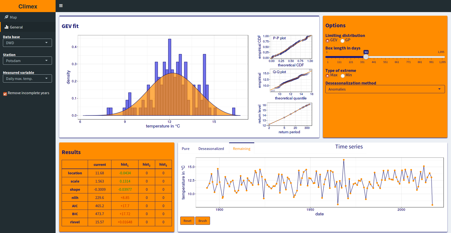
The second tab provides full control over all steps involved in the fitting of the station data via an intuitive GUI in a persistent way (changes will be applied to the analysis of all following time series). You can e.g. pick either the GEV or GP distribution, exclude single points or whole parts of a time series from the analysis, or calculate the return level for the minimum values instead of the maximum ones.
A detailed description of the different features is given in the corresponding vignette.
You are curious and want to try the package or the web application? Using the following link you can test the web application.
Installation
You clone the repository using your command line,
git clone https://gitlab.com/theGreatWhiteShark/climexopen a R shell in the newly created folder,
cd climex
R
and install the package using the devtools package.
devtools::install()Usage
You are new to R? Then check out the compiled list of resources from RStudio or the official introduction.
A thorough introduction is provided for the general usage of the package and the Shiny-based web application, as mentioned beforehand.
When using this package in your own analysis, keep in mind that its functions expect your time series to be of class xts and not numeric!
Update 29.11.2018
Rewriting the post to cover the updated climex version 2.0.0.